Historical NFL Tiebreakers

Untying the standings: the history of the NFL playoff tiebreaker systems

• NFL TIEBREAKERS

  by Ben Austro - December 27, 2018 

Ben seems to have lost his domain but this was tremendous work, and of course very useful to SOM Footballers.

For Michael Paul Payne

SOM PRO FOOTBALL LINKS

Start:

From 1920 to 1931, there was no championship game and the league championship was formalized by a vote of owners at their spring meetings. Unofficially at first, the tiebreaker for the championship favored the latest head-to-head meeting between the tied teams, and presumably working back to an earlier matchup if that game was tied.

In 1932, a tie between the Portsmouth Spartans (today’s Detroit Lions) and the Chicago Bears led both teams to mutually agree to hold a playoff game for the championship. This one-game playoff for the league title was added to the regular-season standings, and actually caused the Spartans to drop to third place with the loss.

A championship game has been scheduled for every season since 1933. Until the Super Bowl era, the winners of the two divisions met for the NFL Championship. If there was a tie in the standings for a division, a one-game playoff would break the tie to determine the team to advance to the championship game, with the home field determined by coin flip. (These games did not affect the standings as the 1932 game had.) In case of a three-way tie, which never happened, there would have been a two-game playoff. A series of coin flips (which occasionally happened) would determine which two teams played first to advance to the playoff game with the third team.

(FJB - my understanding is A would play B and the winner would play C. If the winner of the first match also won the second, then they win the conference or division outright and advance. If not it is possible C would play the loser of the first match and then its net points overall, since C would either have two wins or all three teams would be 1-1.  This was hazily mentioned in newspapers in 1957.)

A one-game playoff was used to break these ties in the standings: (FJB note location determined by coin flip.)

• 1941 Western Division
• 1943 Eastern Division
• 1947 Eastern Division
• 1950 American Conference and National Conference
• 1952 National Conference
• 1957 Western Conference
• 1958 Eastern Conference
• 1963 AFL Eastern Division
• 1965 Western Conference
• 1968 AFL Western Division

Overtime was officially added to the bylaws for the one-game playoffs in 1941, since a team had to advance to the Championship games. The bylaws were amended in 1946 to include sudden-death championship games.

In 1967, the NFL moved to a prescheduled 4-team playoff for the league title. The AFL used a similar format in 1969, prior to merging with the NFL. This began a system of breaking ties through multiple methods, and ended an era of the one-game playoff. The following tables illustrate the various tiebreakers that were in place every season.

(FJB note: ties did not count in the records as a half win and half loss until 1972.  This means a 10-0-1 team and a 11-0-0 team in 1971 have identical records, 1.000.  For this reason I encourage gamers to tie like hell any game they can before 1972, because a loss is far more damaging than a tie, especially against a rival, just ask the 1967 Colts.  Regulation overtime for one period was added in 1974.)

Division

The AFL had a provision to use the division tiebreaker in 1969 to break a tie for the second playoff seed in either division. 

(FJB prior to that only the Division Champion, East or West was awarded a playoff berth in the AFL championship and these were settled by playoff games, i.e. Kansas City and Oakland in the 1968 Western Division. In other words the 1967 and 1968 AFL did not follow the 1967 NFL into divisional tie breakers. But four teams made the playoff in the 1969 AFL).

(Per Tommy Nobis the 1969 AFL matched the East winner hosting the West’s second place team and the West winner hosting the East’s second place team,)

	1967-69	1970	1971-75	1976-77	1978	1979	1980-2001	2002—
1.	Pts ± H2H	H2H	H2H	H2H	H2H/Sweep	H2H	H2H	H2H
2.	>Yrs DIV Title	DIV	DIV	DIV	DIV (skip >2 tms)	DIV	DIV	DIV
3.		CONF	CONF (’75†)	CONF†	COM	CONF	CONF	COM
4.		Pts ± H2H	Pts ± H2H	Pts ± H2H	Loss COM	COM	COM	CONF
5.		*	Rating DIV	Pts ± DIV (avg)	SoS	Pts ± DIV	Pts ± DIV	SoV
6.		Coin flip	Rank DIV	Pts ± CONF (avg)	Pts ± COM	Pts ±	Pts ±	SoS
7.			Coin flip	Pts ±	TD ± COM	TD ±	SoS	Rank CONF
8.				Coin flip	Pts ±	SoS	TD ±	Rank NFL
9.					Coin flip	Coin flip	Coin flip	Pts ± COM
10.								Pts ±
11.								TD ±
12.								Coin flip

Conference

Conference tiebreakers are used to break ties between teams from different divisions. Initially, they were used only to determine a wild card team, but later included conference seeding and home-field advantage as the playoffs expanded.

In most years, if all of the tied teams were in the same division, the tie has been broken using the divisional tiebreakers, even if it is to determine a conference seeding.  1970 and 1978, when the conference tiebreakers were in place exclusively for wild-card ties between same-division teams, were exceptions.

	1970	1971-75	1976-77	1978	1979	1980-89	1990-2001	2002—
1.	1 per DIV (>2 tms)	H2H	1 per DIV (>2 tms)	Sweep	Sweep	Sweep	1 per DIV	1 per DIV
2.	H2H	CONF (’75†)	Sweep	COM (2 min)	CONF	CONF	Sweep	Sweep
3.	CONF	Pts ± H2H	CONF†	SoS	Pts ±	COM (min 4)	CONF	CONF
4.	*	Rating CONF	Pts ± H2H	Pts ±	TD ±	Pts ± CONF	COM (min 4)	COM (min 4)
5.	Coin flip	Rank CONF	Pts ± CONF (avg)	TD ±	SoS	Pts ±	Pts ± CONF	SoV
6.		Coin flip	Pts ±	Coin flip	Coin flip	SoS	Pts ±	SoS
7.			Coin flip			TD ±	SoS	Rank CONF
8.						Coin flip	TD ±	Rank NFL
9.							Coin flip	Pts ± CONF
10.								Pts ±
11.								TD ±
12.								Coin flip

• H2H, DIV, COM, CONF: Win-loss record in head-to-head, division, common, and conference games.
  • If Sweep, then one team in a tie of 3+ teams must have beaten or lost to all other teams in the tie (but head-to-head for 2-team ties)
  • Skip the tiebreaker step if a minimum number of games isn’t met, where indicated
  • Skip the tiebreaker step if it is noted with a dagger† and tied teams haven’t played the same number of games
• Loss COM: Fewer total number of losses in common games (½ for ties)
• Pts ±: Differential in points in all games.
  • When it’s followed by H2H, DIV, COM, or CONF, then the point differential is only in those games
• 1 per DIV: eliminate intradivisional ties first, leaving no more than 1 team from a division in a conference tiebreaker.
• SoV: Strength of victory (aggregate W-L of teams beaten, counting twice if beaten twice)
• SoS: Strength of schedule (aggregate W-L of teams played, counting twice if played twice)
• Rank: Sum of rankings of Points Per Game Scored + Allowed in all games. (A team 1st in points scored + 4th in points allowed has a rank of 5.)
  • When it’s DIV or CONF, then it applies to ranking within the division or conference teams, but counting all games
• Rating: Similar to the Rank method, but instead of all games, it only applies to points per game in division or conference games, whichever is indicated
• TD ±: Differential in touchdowns in all games, or in common games where indicated
• * The tiebreaking procedures put in place before the 1970 AFL-NFL merger included a step that would eliminate the team that was most recently in the postseason. However, the procedure specifically stated this step was not in force for the 1970 season. Before the 1971 season, the tiebreakers were revised, so this provision was never officially in place.
• >Yrs DIV Title: prior to the merger, if the head-to-head point differential was 0, the division champion would be the team that went the longest without a division title.

Note that a W-L record disregarded tie games prior to 1972, so a 4-1-1 record calculated only the 5 untied games (4 ÷ 5 = .800). Since then, ties count as a half-win (4½ ÷ 6 = .750).

In the 1982 strike season, teams were seeded 1-8 for a modified playoff tournament using the conference standings only. Division standings and tiebreakers were not used that year.

Source: https://web.archive.org/web/20211204130343/http://www.quirkyresearch.com/2018/12/27/untying-the-standings-the-history-of-the-nfl-playoff-tiebreaker-systems/?replytocom=16569

One Last Time with Team Interceptions, Part 4

 One Last Time with Team Interceptions, Part 4

SOM PRO FOOTBALL LINKS

So, the question came up- why not generic team charts, like/ similar to batting cards?

Let’s look first at the problem batting cards were trying to solve.  Take a Sixties baseball team and the pitchers (in sum) will bat about as much as 2/3rds of a regular, and mostly not very well.  But you get exceptions.  When you try to cut a team’s total pitcher batting into the individuals you eventually get a handful of relief pitchers who banged a triple in five at bats, or a homer in ten at bats, and unless you were Earl Wilson in 1968 a personal card reflecting this this is somewhat unrealistic. 

Most pitchers stink when batting so (other than personal cards) there are two ways to solve this – you can aggregate the whole team (a method I use in Statis-Pro Baseball, which is going to have the effect of grouping a pitcher with no power like Mickey Lolich in with Earl Wilson) BUT it is just easier to manage and works for probably 25 out of 28 teams.   Or you can group the pitchers by type.  This is what Strat-O-Matic did, first with four pitcher’s batter’s cards, and then with eight during the baseball card game’s Golden Age.   

They chose five cards for pitcher with no power, and three for pitchers with power:

IF NO HR'S OR AB/HR>=68 

Bavg           Card 

.000 - .134      1 

.135 - .179      2 

.180 - .224      3 

.225 - .269      4 

.270 +             5

 

 

IF AB/HR < 68 

Bavg           Card 

.000 - .199      6 

.200 - .249      7 

.250 +             8 

 

One look and you can see the first five cards are probably reasonably spaced; this is probably not a bad way to model pitchers with no power. No, it won’t accommodate pitchers with a lot of walks or extra base hits past a certain point but those are rare anyway.  It is the last three cards that bother me, that range for Card 6 is from truly lousy pitcher’s hitters who catch hold of one (here’s looking at you, Bartolo Colon) to pretty good hitters who might have reasonable power, like Dave McNally or 1972 Bob Gibson.  That range is too broad for Card 6.  Now- does it matter? 

Well SOM baseball fan Flying Pickle actually put all pitcher’s batting cards in a spreadsheet about fifteen years ago, and here were the results:

 

Figure 1: Pitchers Batting Cards, 1901-2008

There aren’t that many Card 6 guys anyway, and what would they get? For a number one starter maybe 40-50 AB?  Cards 6-8 are less than seven percent of all pitchers who bat.  The question of whether there ought to be ten or twelve pitcher’s batting cards (more than eight) is mooted by the fact these players are peripheral to their team’s overall offensive experience.   Most players will want the simpler answer or the most complex, i.e.  individual cards.

And that brings us to Team Interception Returns.  I’m pleased that I finally got the last two teams from 1980 to finish my Wideboys collection; this final event was over a year in the making.  I might be poorer, but I sure have a smile on my face, because I’ve been horsing around now for a day or two with this season’s cards in my off time.  One might say I have 1980 on my mind. Two of my favorite teams are 1980 LA and 1980 Dallas, the Wild Card runts of the 1980 NFC despite good records.  1980 LA is an offense first team with one of the team’s weaker run defenses of the last decade, they finished with a pretty good turnover plus minus but with terrible kicking.  They still got 405 points even with Haden in for fifty attempts, more than ten percent.  The Cowboys led the 1980 NFL in scoring in spite of having the ninth best offense in yards. Dallas had Tony Dorsett push for 11 TDs and 1185 yards on the ground while five other runners chipped in 991 yards and another ten TDs. Dallas scored like this year’s Detroit Lions, but in one less game, and the Rams were not far behind, even though neither team made a lot of kicks. What was setting them up?

Aha!  The 1980 Season’s interception returns helped to define the 1980 season!

Figure 2: A sampling of team interception returns by team from the 1980 season:

The World Champions and two of the ten playoff teams are in the top yardage tier, teams that averaged more than thirty yards of interception returns a game.  The next tier is limited more by opportunities, as Denver would have led the league in yardage had they matched the Oakland interception total.  Still, we see another three playoff teams there, and only one team, Philadelphia in the bottom tier.  This is not uncommon.  LA and Dallas might have been 10-6 type teams had their returns not elevated them to 11-4 (with Ferragamo) for LA and 12-4 for Dallas. Their team returns were not peripheral to their success, they were the key to it. Another way to look at it is Atlanta, also 12-4, was plus sixteen in turnovers and had great special teams, a plus kicker in Mazzetti, a good punter in James, good coverages, and a top three punt return unit.  All that offset an iffy pass defense. Why shouldn’t Dallas and LA get the same boost from their secondaries?

One last point I’ll make is the seasonal record even at first blush for each team holds a lot of information.  Let’s look at 1980 Dallas- the first rung of data that you see in PFR:

Figure 3:  1980 Dallas Return Results First Pass from PFR: (Click to make bigger)

So, we have the longests.  And if a guy has two returns with a longest of 2 yds that means the other return is a zero.  If a guy has 3 returns for 56 yards with a longest of 56 yards the other 2 are zeros.  Just at first glance you have half of the returns and you can guess they might be “chunky”.

Looking up the weekly records by player for Thurman, Waters, Breunig, and Wilson finishes the record.  Thurman’s best day saw him get two for 42 yards with a longest of 35.  That means the other is seven yards.  Here’s how it fills out:

Figure 4: 1980 Dallas Final Record

And this is the Team Card from the Game:

Figure 5: 1980 Dallas Returns

I could see maybe adding in that 56 yarder in the twelve spot and cutting the +12 yard result in the seven spot to +9 but that increases the fractional TD pct by a few points, so I didn’t do that.  You can see the chunky nature of the team’s returns in the nine 30 (or so) yard chances they have out of 36.   In the final analysis once you get this close it’s not going to matter, Mike might do better with his reckoning, but it’s a pretty good chart. Taking into account returns “not returned using the rule for that” for 0 yards this chart is manifestly better at describing 1980 Dallas than the stock chart.

We’ll put one last chart up there, 1980 Seattle:

Figure 6: 1980 Seattle Seahawks Team Card (23/95 yards, 0 TDs, 4.1 yds per return)

I’ll let gamers be the judge as to whether or not a generic chart is a better fit for this team’s efforts.  In my opinion, though, team interceptions are more like running cards then baseball’s pitcher batting cards, where there can be many ways to get to the final rushing stats line. If there weren’t we could just use the extra runners from the set of extra player cards and change a few results to make a season.  And, of course, we don’t do that. We can do better than that.

 

Fred Bobberts

Initial Date of Publication: 2/10/2024

PS - I'm not going to spend one more minute of my time on this.  If you don't like the feature, turn it off.  I'm done feeding the trolls.

The (Second to the) Last of Three (no, Four) parts on the Team Interception Feature in Strat-O-Matic Pro Football.

 The second to the Last of Three oops four parts on the Team Interception Feature in Strat-O-Matic Pro Football.

 

 The real-life 1970 Lions scored 4 TDs on 28 interceptions.  Is this better or worse than expected?

SOM PRO FOOTBALL LINKS

“Sometimes, the season itself is the outlier”

 –Scott Everngam

 In the previous installments, we explored the design intent of the feature, and the challenges in evaluating the raw interception return data a season might produce. We’ve shown the feature is pretty good at distributing the most return yards to the most threatening teams; in as few as six replays real trends start to appear that mirror real life team results.  We’ve show it is an improvement over the stock interception chart.  But we haven’t tackled the final objection- why is it a season like 1975, which had 533 interceptions but only 25 interceptions returned for TD, or 1977, which tallied 562 interceptions but only 28 returned for TD will come out consistently high when using this feature? 

Well to look at this, I created a graph of every season’s Real Data from 1956 to 1981, effectively bracketing these years, plotting the season’s overall interception return yardage average and pct of overall interceptions returned for TDs.  And while the fit is not perfect, it is not exactly a random walk, either.  At the season level, the best fit for TD pct vs return average over the range of data we see is a second order power law, implying a fairly strong push upward in “house pct” as the average yardage per return increases.  And here it is:

Figure 1: Season Level Real Life Data for Average vs TD PCT, 1956-1981

This is all real NFL Seasonal data compiled from each team’s data underneath it, except for the 1975 replay data point the original chart data points in red.  The original chart was developed in 1968 for the game’s initial release and very much is a product of its time; it reflects the five seasons in the mid-Sixties that surround it.   1975 and 1977 in real life were below the curve of expected TDs their yardage would have normally produced, with 1975 in particular about 1.8 pct lower than predicted for its 14.5 yards per return.   Over 533 interceptions this would produce a deviation of 8-10 interceptions versus a typical such season over NFL history.  The effect in 1977 is less pronounced but probably still about 7 interceptions low.  The Fifties teams and quite a few mid Seventies teams are low outliers, while the mid to Late Sixties trend high.  Sometimes the real data from the season itself is the outlier, as Scott observed once while creating CMs.

It’s a pat answer but I haven’t explained why this is true. It’s a heck of a lot of data, if this were a normal distribution 26 seasons and 13,095 interceptions should produce a pretty nice chart, not the messy correlation we see above.  But the overall data set is neither continuous nor normal; the y axis response is low frequency binomial (yes/no) data, and each season is a collection of subsets of team data that lie beneath its sums.  If you look at the team data over the same period, you see it has some very interesting properties:  

Figure 2: Team Level Data, Aggregated by Range

There are no seasons that sum out as low as the lowest team ranges or as high as the highest team ranges.  Seasons are populations of teams. At the team level both the TD percentage and the percentage of 0 TD returns in the sample range are strongly correlated to the average yards per return. The latter case is in the inverse, as teams with interception return averages less than 12.0 will fail to get even one TD more than half the time.  It’s important to note that even real-life teams that had very high return averages might fail to tally even one TD in one out of eight (or so) cases.

Another way to look at it is 18 pct of teams had 17 yds or greater per return; these teams accounted for 25 percent of the total yards and 30 percent of the total touchdowns during this interval.  Six out of seven of them with have at least one TD, as opposed to two thirds of the total.

I keep harping on these high average teams because they help to explain why certain higher average return seasons have such high variability.  Season such as 1975, which averaged in the mid 14 yards per return range do not have every team as a high performer.  Instead, a higher seasonal average is more an indicator that there are also some high potential teams mixed in with the rest of a typical population, rather than a guarantee of high return touchdown percentages.  If we return to the original chart, we see three teams had similar overall return avg stats but different TD percentages (again real-life data):

Figure 3: Team Level Data for three NFL seasons in the mid 14s for average yard per return

  

That’s quite a range of TDs and House Pcts from a narrower range of inputs, but actually all three are possible based on the underlying data, which is decidedly not continuous nor normally distributed.  There is no guarantee that a team with a high return average will meet its potential and no guarantee that a team won't uncork a TD when the rest of the real-life teams with similar averages mostly didn't. 

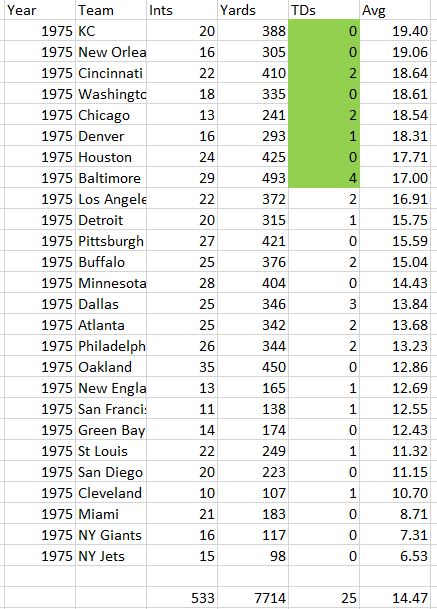
Looking at 1975 we see that other than Baltimore that key team population at/or/over 17 yards a return is not carrying its weight in TDs, with four teams out of the top eight not getting any at all.  That number should be one out of eight when considering NFL History, so this type of distribution will happen about 1/80 times. Unlikely, but not impossible.

Figure 4: Team Level Data for 1975

Now we look at the middle season, 1971.  Led by Houston the top teams get 12 return TDs in 115 returns.  Washington, which is in the next range subpopulation down, also chips in a nice year:

Figure 5: Team Level Data for 1971 

And, finally, the high field, 1966.  Here the top teams are robust and are also supported by good seasons from Miami, Buffalo, and LA.  This outcome is also merely unlikely, but not impossible:

Figure 6: Team Level Data for 1966  

In summation, some corrections on team charts can be made to try to tame high observed interception return TDs. But there are limits on how far you can go, and to how much these adjustments will translate in seasons with higher return averages. Throughout NFL history, it can be shown that there is a strong correlation between team interception return average and the percent of these interceptions returned for touchdowns.  And the goal of the feature is to closely match relative return yardages within a season, if fed the same number of interceptions per team. 

It is also possible that the season itself is an outlier when its combined team population's results are compared to all teams in NFL History.  One must consider what the predicted outcome is likely to be, not just a deterministic idea of what a statistic should be based only on a value, and not within its context.

Note: the original questions on the Forum concerned 1977, which is why I mentioned it.  But, unfortunately, I don’t own 1977 to test in detail, so I chose 1975 to illustrate the point.  Teams like 1975, 1977, 1979 and 1981 are all somewhat analogous, while the mid to late Sixties are also analogous on the high side.

Fred Bobberts

Original Publication Date: 2/4/2024

1967 AFL “Wideboys” Player’s Aids For Strat-O-Matic Pro Football - Original Cards

 

Abner Haynes shared time with the 1967 Miami Dolphins and New York Jets

New! Improved! Analysis below!

SOM PRO FOOTBALL LINKS

1967 AFL “Wideboy” Cards for Strat-O-Matic Pro Football,

Including Updated Special Teams, Penalties, and Extra Players. It is 85 new sides, about a quarter of the AFL season of new content.  You should be able to print these off Landscape on A4 and while they are not an exact match, size wise, they’ll work for gameplay. 

1967 AFL Players List (Drop Box Link) :

1967 AFL Players.pdf

20 extra players, at least one for each team, with some teams having as many as three.  Consult this table for potential block ratings. 

1967 AFL Extra Player Cards (Drop Box Link) :

67AFLExtraPlayers.pdf (21 Player’s Cards in PDF format)

It should be noted I’ve left some Year One only card quirks in, like the absence of QB double team completions, and certain results where defense right is greater than defense wrong for a few split numbers for runners on certain teams. I figure Hal might have wanted them that way. 

67AFLPuntKickCards.pdf

The original method of carding Field Goals is, to me, unplayable. Towards the late Seventies the Game Co. started to “blend” results if there was a longer range with better percentages than a shorter range, which meant you didn’t have to take a knee to lose five yards to set up a longer kick at a better probability. I will say you can use the old kicking cards with the new plus minus five yard rule and they kick a lot better but these kickers I’ve made can adhere to the bylaws of the time. 

Note that the yardages reflect the 1-12, 13-22, 23-32, 33-42, 43-47 scrimmage lines of the time and you subtract 10 yards from these spots if playing another Wideboy team from 1974 on. 

These cards include penalties, team carding for punts, and kick and punt coverages. They are different than the cards in the updated PC game, as a different model was used there. 

67AFLReturnCards.pdf

Summary:

The AFL's best overall special teams belong to the 13-1 Raiders, with Blanda as an excellent kicker, good return coverages and punting, and solid returns.  The AFL does not have the kick returners the NFL had, but Denver can return punts as well as anyone.  

Analysis:

1967 Boston Patriots

Special teams:

Swanson could use more punt yardage, but the return coverages are pretty good (especially against punts) and Gino Cappelletti can nail kicks at 2-7 all the way out to 49 yards, and Jay Cunningham is sneaky as a #2 punt returner. Cappalletti would retire after 1970 as one of only three men with over a thousand points in Professional Football History (1,130) and with the most points in AFL history (1,100).      

Personnel:

Added John Huarte’s 9 pass attempts as a QB, HB JD Garrett, and Tony Romeo’s 1 rated blocking TE card.

 

1967 New York Jets

Special teams:

The Jets give up a long gain on punt return defense but are otherwise sound, above average both against kicks and punts. Curley Johnson is a good punter with no blocks. Jim Turner had a bit of an off year, only 2-10 on extra points and his range really drops off after 40 yards. Bill Baird and Earl Christy are average on punt returns with the ten and four spot fumbles (a Seventies era occasional head-slapper for teams with low fair catches) and the kick returns are just so-so. I subbed in Emerson Boozer for Abner Haynes for KR #2 since Haynes is now “returned” to Miami.    

Personnel:

I gave the Jets FB Billy Joe and the ability to trade back Abner Haynes to Miami. You’d think the addition of a 37 carry runner wouldn’t matter much, but if you try a 1967 Jets replay (as I am doing) you hit the wall on carries real quick, especially late in the season if you trade Abner Haynes back to Miami:

1967 Jets Carries by Runner and Availability by Game

 

This grid shows the real-life availability of each runner from the rushing records, and it shows why 1967 Namath had to throw as much as he did. Boozer was actually an AFL All-Star off of what are seemingly middling stats (442 rushing yards and 205 receiving yards) but he led the AFL with 13 TDs (and 10 on the ground) and accomplished everything he did in only 8 games. Meanwhile Snell was missing in action after the first game, returning for Game 9 onward.  But after the third game, the Jets are scrambling for team carries, and while real Pro Football teams do not have Strat-O-Matic football attempt limits it is easy to see that they were hurting.  A late trade with Miami gave them Abner Haynes, and that is how Hal carded the Jets in Year 1- Snell, Smolinski, Boozer, Mathis and Haynes, not giving Mathis a FB/HB rating which would have helped.  But that would also allow his to be a receiving FB, Smolinski’s role, so I can see why he carded the positions the way he did. In that context, Billy Joe’s added extra carries at FB certainly help.

A cards and dice gamer has a choice for a 1967 Jets replay – rotate the carries around a version of the “per 14” row number, or in the case of the utility, where you are limited to four backfield runners, let Joe be the FB and Smolinski back him up for games 2 through 8. If you don’t let the Jets have Haynes, you will need to be creative from Game 9 on, since you will have only Bill Mathis (albeit a great receiver) at HB. Easy to see why they faltered down the stretch, and if you check Game 11, a 33-24 loss to the hapless 2-10 Broncos, you find the three runners they had mustered only 9 carries among them out of the backfield for 40 yards, forcing Namath to throw 60 passes in a game they trailed 33-3 at one point.

The other player added to the 1967 Jets is Curley Johnson as a backup TE, something Mike Kane had caught for the recards.  Since Hal carded 5 RBs in the 11 positions, he also used George Sauer as the backup TE with a block of 0.  But Johnson was a RB/TE type earlier in his career, with 26 carries and 14 catches as recently as 1962, so he’s on the extra player list as a TE with a block of 1 for goal line situations.   

 

1967 Buffalo Bills:

Special teams: 

Paul Maguire is a great punter with good coverages, and Mike Mercer is better than most at hitting long field goals.  Buffalo has a minus seven penalty ratio, though, and none of the return men are very good.

Personnel:

Added Jack Spikes and Ed Rutkowski, mostly fringe players.

 

1967 Miami Dolphins:

Special teams: 

Larry Seiple punts for good yardage, even with a blocked punt.  The Dolphins have excellent punt coverage but the kickoff coverage lags.  They are plus three on penalties. Booth Lusteg is a sub-par kicker.  The kick and punt returns are fairly average.

Personnel:

As noted in the Jet’s section, Miami gets Abner Haynes and his second on the team 56 carries back. The Dolphins also get carries from their quarterbacks, particulary Griese, but they needed backfield help.  Note that this goes beyond just changing the team name on his card; the team’s blocking ratings for the offensive line and different fumble range must also be added.  The Dolphins add a fringe wide receiver in Frank Jackson and a third quarterback in Archie Roberts.  His one game career is now memorialized in his lone SOM passing card. The re-addition of Haynes does make them more playable.

 

1967 Houston Oilers:

Special teams: 

Kicker John Wittenborn loses his range after 30 yards, but he hits all his extra points, and Jim Norton is a good punter for average, minus the block on twelve.  Larry Carwell makes a nice PR #1 and Zeke Moore has a KR TD in the 11 spot as KR #2.  The Oilers are the best KR defender in the 1967 AFL but punt coverage is average.      

Personnel:

Glenn Bass and Larry Elkins are fringe receivers.

 

1967 Denver Broncos:

Special teams: 

Bob Scarpitto can punt for distance, but he has a block in the 12 and the Bronco punt and kick coverages are among Pro Football’s worst.  Bob Humphreys is a poor kicker. But Denver Special teams mean you get Floyd Little, and he is a great punt returner, with a TD on 3, and kick returner, even if the #2 guys let the side down a bit.

Personnel:

Unfortunately Scarpitto (WR), Fran Lynch (RB) and Cookie Gilchrist are mostly fringe players.  For Gilchrist this was his last card, as he retired having led the AFL in carries three times, rushing yards twice, and rushing TDs four times in his short but brilliant career.

 

1967 Kansas City Chiefs:

Special teams: 

Jan Stenerud fell off a bit on longer (33-42 yd line) kicks, but he stll nailed the most touchbacks.  Jerrel Wilson has decent punt yards but a block on 12.  They give up a LG on kick returns and the punt coverage is below average. But they have Noland Smith, a capable punt returner and an excellent kick returner.  Smith has a TD in the 2 spot on kick returns.

 

Personnel:

The lone Kansas City extra player, Frank Pitts, doesn’t catch many but when he does, look out.  He has some Long Gains on his card and averaged over 30 yards a grab, albeit on limited touches (4).   

 

1967 Oakland Raiders:

Special teams: 

One way to win 13 games and lose only one is to feature the best special teams in your league.  Punter Mike Eicheid kicks for great yardage, albeit with a block in the 12 spot. But he is backed with great punt return yardages, and the kick coverage is above average, too.  Kicker George Blanda is a real weapon, too- 2-7,12 out to the 42 yard line, 2-11 on extra points, he is the All-AFL kicker.  Rodger Bird is a good punt returner, and the kickoff guys are solid.  No real weaknesses, with Blanda a big strength.

Personnel:

Another trick is to be deep off the bench.  Dave Kocourek, a sub TE, picks up a 2 block rating, and the running game gets a boost from HB Larry Todd, who adds 29 serviceable carries to an already strong backfield.

 

1967 San Diego Chargers:

Special teams: 

The Chargers’ return coverages were not great, but Dick Van Raaphorst was a 70 plus percent kicker inside 40 yards and Rick Redman escaped the punt block hex. At least they don’t give up Long Gains.  Speedy Duncan is a great punt returner, though, and the Chargers get above average kick returns from both Jim Tolbert at #1 and Dickie Post at #2.

Personnel:

The original cards have two wonderful runners, Brad Hubbert and Dickie Post, both All-AFL, but Gene Foster and Paul Lowe are sub-par running substitutes.  Russ Smith and Jim Allison give San Diego 32 useful carries to back up Hubbert, who had only 116 for the year at FB.    

 

A ‘68 will be on the way, probably later this year. 

Fred J. Bobberts 

Original Date of Publication: January 15, 2024